


In 2017, the City of Winnipeg wanted to get some solid numbers about how much traffic was actually delayed at this crossing. The City approached TRAINFO and asked for our help. We happily agreed and used it as an opportunity to compare the conventional modeling method and TRAINFO’s new measurement method for estimating traffic delay at rail crossings (these methods are explained in detail in an earlier post here).
Over a 91-day period (August 1, 2017 to October 31, 2017) we collected data to use for both these methods. This post describes and compares the results of these methods.
About the Waverley St Rail Crossing
Waverley St is a major north-south urban arterial roadway with two lanes per direction, an average daily traffic volume of 33,665 (about 16,832 per direction), and a posted speed limit of 60 km/h near the crossing. There is a double-track railroad crossing close to Taylor Ave. The railroad is a mainline track that has an average of 35 through trains per day and a maximum train speed of 35 mph. Figure 1 shows a picture of this crossing and the traffic queue during a blockage.
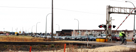
Figure 1: Waverley St Rail Crossing and Traffic Queue
The Math Behind the Methods
The Modeling Method: The basic equation for calculating total vehicle delay per train using the modeling method is:
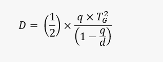
Where,
D = total vehicle-delay per train (minutes)
q = vehicle arrival rate (vehicles per minute)
TG = gate downtime (minutes)
d = vehicle departure rate (vehicles per minute)
For this study, we assumed the following:
- Average train length = 7,000 ft (industry average)
- Saturation flow rate = 1,900 vehicles per lane per hour (traffic engineering theory)
- Advanced warning time = 20 seconds (industry average)
- Clearance time = 10 seconds (industry average)
- Train volume = 35 trains per day (given by Transport Canada)
- Avg daily traffic volume = 16,832 vehicles per direction per day (given by City of Winnipeg)
- Total traffic volume over 91 days = 1,531,712 (calculated as 16,832 vehicles per day x 91 days)
- Total blockages = 3,185 trains (calculated as 35 trains per day x 91-days)
- q = 4.68 vehicles per minute (calculated as 16,832 vpd ÷ 3,600 min/day)
- d = 63.3 vehicles per minute (calculated as 1,900 vplph x 2 lanes ÷ 60 min/hr)
- TG = 2.8 minutes (calculated as 7,000 feet ÷ 35 mph + 20 s + 10 s)
The Measurement Method: The basic equation for calculating total vehicle delay per train using the measurement method is:
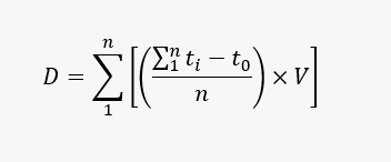
Where,
D = total vehicle-delay per train
t0 = expected travel time with no train (as measured by Bluetooth sensors)
ti = actual travel time of vehicle, i (as measured by Bluetooth sensors)
n = blockage event (as measured by train detection sensor)
V = number of vehicles impacted by the crossing delay
For this study, we collected rail crossing blockage data with TRAINFO’s train detection sensors and vehicle travel time with Bluetooth sensors over a 91-day period. This data was plugged into our machine-learning algorithms and proprietary software to directly measure individual vehicle delay at the rail crossing with and without a train. No assumptions!
Results, Drumroll Please
The Modeling Method: Plugging in the data, we calculated the following vehicle-delay per train:
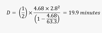
Therefore, according to the model, the total vehicle-delay over 91 days is 63,110 minutes (calculated as 19.9 minutes per train x 3,185 trains and the average delay per vehicle is 2.4 seconds (calculated as 63,110 minutes ÷ 1,531,712 vehicles x 60 seconds/minute).
The Measurement Method:
Over a 91 days data collection period, we detected 3,422 rail crossing blockages (including through trains, switching movements, equipment malfunctions, and all other instances where the crossing was blocked), and an average gate downtime of 5.9 minutes. We measured vehicle-delay per train as 86.7 minutes, total vehicle-delay of 528,005 minutes, and average delay per vehicle of 20.4 seconds.
Further, the measurement facilitated much deeper analysis and understanding of traffic delay at rail crossings. Figure 2 shows a probability density function that provides the distribution of crossing blockages based on the blockage duration and the vehicle-delay caused by these blockage durations. Total vehicle-delay is represented by the area under the “Minutes of Vehicle Delay” curve (orange line).
Here’s an example of how to read this figure. This figure shows that there were about 225 blockages with a 10-minute duration (blue line, left vertical axis). These blockages combined to cause about 80,000 minutes of vehicle-delay (orange line, right vertical axis).
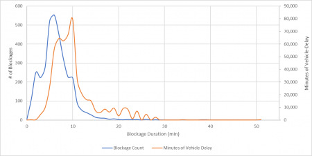 Figure 2: Probability density function of number of crossing blockages and minutes of vehicle-delay based on the measurement method
Figure 3 shows the same data except plotted as a cumulative density function. Here’s an example to help read this figure. This figure shows that blockages lasting 10 minutes or less cause 70% of total vehicle-delay.
Figure 3: Cumulative density function of total vehicle-delay and crossing blockage duration based on the measurement method
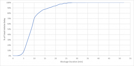
Figure 3: Cumulative density function of total vehicle-delay and crossing blockage duration based on the measurement method
Key observations revealed by these figures include:
- A small number of very long blockages cause more delays than many short blockages (Figure 2). For instance, the 23 longest blockages, representing those of 19 minutes or longer, caused more delay than the 1,385 shortest blockages, representing those of 5 minutes or shorter. Therefore, a significant amount of traffic delay can be addressed if long blockages can be predicted to re-route drivers around the crossing.
- A large proportion of vehicle-delay is caused by a relatively small number of blockages (Figure 3). For instance, 30% of total delay is caused by 15% of blockages (i.e., blockages of 10 minutes or longer).
- The average gate downtime is a poor indicator of blockage duration (Figure 3). For instance, the average gate downtime for the modeling method (i.e., 2.8 minutes) and the measurement method (i.e., 5.9 minutes) only accounted for 1% and 10% of total vehicle-delay, respectively.
Side-by-Side Comparison
The Measurement Method is based on ground truth data and significantly outperforms the conventional modeling method. Overall the measurement method finds that traffic delay at the Waverley St crossing is more than 700% higher compared to the conventional method. Table 1 compares key metrics between each method.
Table 1: Comparison of key performance metrics between the conventional and new method
| Metric | Conventional Modeling Method | TRAINFO Measurement Method | Percent Difference |
| Number of blockages (over 91 days) | 3,185 | 3,422 | +7.4% |
| Total blockage duration (over 91 days) | 148.6 hours | 336.5 hours | +126.4% |
| Average vehicle-delay per blockage | 19.9 minutes | 86.7 minutes | +335.7% |
| Average delay per vehicle | 2.4 seconds | 20.4 seconds | +750.0% |
| Total vehicle-delay (over 91 days) | 1,052 hours | 8,800 hours | +736.5% |
Conclusion
Until recently, the conventional Modeling Method was the primary approach for quantifying traffic delay at rail crossings. TRAINFO’s new, affordable technologies are providing a superior alternative to help truly understand traffic delays at rail crossings. This understanding helps traffic engineers confidently respond to public complaints and prioritize investment strategies.
Here’s one way the Measurement Method can help. Imagine applying for federal funding to construct an underpass at a rail crossing. Chances are high that you will need to include a benefit-cost analysis to support this application. Based on the comparison described in this post, the Measurement Method would provide a BCA ratio that was SEVEN times higher than using the Modeling Method. For nearly the same cost and effort, you could drastically increase the likelihood of getting federal funding.
And that’s why your traffic model is (probably) letting you down at rail crossings!
References
[1] Chicago Metropolitan Agency for Planning, “Highway Capacity Measurements: Grade Crossing Saturation Flows,” 2015.
[2] J. Appiah and L. Rilet, “Microsimulation Analysis of Highway-Rail Grade Crossings: A Case Study in Lincoln, Nebraska,” in IEEE/ASME Joint Rail Conference, Wilmington, DE, 2008.
[3] J. Powell, “Effects of Rail-Highway Grade Crossings on Highway Users,” Transportation Research Record: Journal of the Transportation Research Board, no. 841, pp. 21-28, 1982.